Computational Observation by NOAA:
Fully describing the carbonic acid system requires that, in addition to temperature and salinity, at least two of the carbonate parameters (pCO2,sw, AT, DIC, pH) be known. To achieve this, NOAA compute daily fields of total alkalinity (AT) and carbon dioxide partial pressure (pCO2,sw) through the application of a variety of modeled and remotely sensed environmental parameters. Sea surface pCO2,sw is estimated using an empirical model relating the differential between sea surface and atmospheric CO2 partial pressure (ΔpCO2 = pCO2,sw - pCO2,air) to changes in CO2 gas solubility (K0). Sea surface AT is derived using the empirical relationships offered by Lee et al. [2006] describing (sub)tropical surface AT as a function of SSS and SST. Monthly composites of these AT and pCO2,sw fields are then coupled to solve the carbonic acid system using the CDIAC Program for CO2 System Calculations [Lewis and Wallace, 1998]. The carbonate equilibria calculations used the Mehrbach et al. [1973] formulations of the K1 and K2 dissociation constants as refit by Dickson and Millero [1987]. A more detailed describtion of the methods employed are given in Gledhill et al.(2008).

Fig1. Methodology flow chart
Monthly composites of SST, SSS, pCO2,sw, and AT are used as inputs to the CDIAC CO2 System Program to solve for the carbonic acid system and obtain maps including carbonate ion and aragonite saturation state (see the flow chart above).
Monthly composites of SST, SSS, pCO2,sw, and AT are used as inputs to the CDIAC CO2 System Program to solve for the carbonic acid system and obtain maps including carbonate ion and aragonite saturation state (see the flow chart above).
Computation of Sea Surface pCO2 and sw Fields:
Sea surface pCO2,sw is computed as a function of CO2 gas solubility using an regionally specific empirical relationship according to (Gledhillet al., 2008):

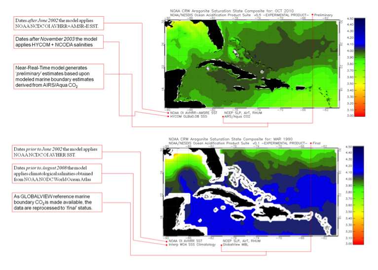
Where yo = -51.2 ± 0.3, A = 350.7±12.3x10³, B = 30.3±0.1x10⁻² for oceanic surface waters of the Greater Caribbean. The temperature and salinity dependent gas solubility coefficient (K0, moles kg-1 atm-1) is calculated according to Weiss [1974] in Near-Real-Time using the 1/4-degree gridded fields of daily NOAA NCDC OI AVHRR + AMSR-E SST OI.2(henceforth referred to as SSTOI) and HYCOM+NCODA SSS. Archived data generated for dates prior to November 2003 were generated using climatological salinities obtained from NOAA NODC World Ocean Atlasand for dates prior to June 2002 the model applies NOAA NCDC OI AVHRR SST
Atmospheric CO2 partial pressure (pCO2,air) is computed according to:

where air pressure (SLP-pH2O) is calculated as a function of air temperature, relative humidity and sea-level pressure (SLP) obtained from NOAA NCEP and calculated according to best practices (Dickson et al., 2007; SOP 5). The dry atmospheric CO2 mole fraction data (XCO2) are based upon the NOAA Earth System Research Laboratory GLOBALVIEW-CO2 reference marine boundary layer (MBL). The GLOBALVIEW marine boundary layer represents a data extension and integration as described by Masarie and Tans (1995) and exhibits considerable latency as flask CO2 data need to be quality controlled prior to processing. This latency can be greater than one year.
Therefore, the Near-Real-Time model generates 'preliminary' estimates derived from the Atmospheric Infrared Sounder (AIRS) mid-tropospheric Carbon Dioxide (CO2) Level 3 Monthly Gridded Retrieval, from the AIRS and AMSU instruments on board of Aqua satellite. While the AIRS/Aqua CO2 retrievals do not measure the marine boundary layer as they represent concentrations primarily from 6-10 km altitude, the bias between the AIRS/Aqua CO2 values and the GLOBALVIEW-CO2 reference marine boundary layer is found to vary in a predicable fashion as a function of time of year and latitude. We have modeled this difference using an amplitude version of the Gaussian peak function over the latitudinal domain of 0N to 53N. The equation takes the form of
Therefore, the Near-Real-Time model generates 'preliminary' estimates derived from the Atmospheric Infrared Sounder (AIRS) mid-tropospheric Carbon Dioxide (CO2) Level 3 Monthly Gridded Retrieval, from the AIRS and AMSU instruments on board of Aqua satellite. While the AIRS/Aqua CO2 retrievals do not measure the marine boundary layer as they represent concentrations primarily from 6-10 km altitude, the bias between the AIRS/Aqua CO2 values and the GLOBALVIEW-CO2 reference marine boundary layer is found to vary in a predicable fashion as a function of time of year and latitude. We have modeled this difference using an amplitude version of the Gaussian peak function over the latitudinal domain of 0N to 53N. The equation takes the form of

Where the standard year fraction (SYF) is simply the decimal fraction of the year (e.g. 0.0 = January 1 and 1.0 = December 31) and the fitting parameters (y0, A, w, and xc) modeled as a function of latitude using polynomial fits. Best fits were facilitated using OriginPro 8 SR5 v8.0897 software.
As updates to the GLOBVALVIEW-CO2 MBL are made available, the data are reprocessed to 'final' status.
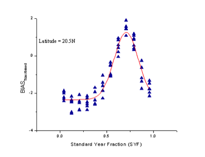
For 'preliminary' estimates of atmospheric CO2 mole fraction data (XCO2) the model estimates the marine boundary layer based upon AIRS/Aqua Level 3 mid-tropospheric CO2. Shown here is the bias between the GVMBL and AIRS/Aqua CO2(2003-2009) modeled as a function of year fraction at 20.5N.
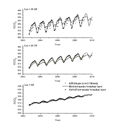
The model performs best at lower latitudes and is applicable only to the domain 0N to 53N beyond which the relationships degrade. At 0N the model exhibits an adj.-r2 = 0.98 (RMSD = 0.63 µatm); 26.7N the model exhibits an adj.-r2 = 0.99 (RMSD = 0.56 µatm); 40.5N the model exhibits an adj.-r2 = 0.98 (RMSD =0.81 µatm); 58.2N the model exhibits an adj.-r2 = 0.92 (RMSD = 1.9 µatm). Shown here is the time-series of the GVMBL (black triangles), the AIRS/Aqua CO2 values longitudinally averaged (grey crosses), and the marine boundary layer as modeled from AIRS/Aqua (black line).
Computation of Sea Surface Total Alkalinity Fields:
Estimates of sea surface total alkalinity (AT) were derived according to the relations offered by Lee et al. [2006] for surface waters using a simple empirical equation of the form:
AT = a + b(SSS - 35) + c(SSS - 35)2 + d(SST - 20) + e(SST - 20)2
To compute daily fields of AT the (sub)tropical form of the algorithm was applied to SST and SSS datasets as described under the sea surface pCO2,sw methods and detailed in Gledhill et al. [2008].
AT = a + b(SSS - 35) + c(SSS - 35)2 + d(SST - 20) + e(SST - 20)2
To compute daily fields of AT the (sub)tropical form of the algorithm was applied to SST and SSS datasets as described under the sea surface pCO2,sw methods and detailed in Gledhill et al. [2008].
Evaluation of Computed Fields:
Daily computed fields have been compared against bin-averaged (1/4° x 1/4° x daily) geochemical cruise datasets from 1997 through 2006 where sea surface carbonate chemistry parameters were measured. For pCO2,sw this includes all the Explorer of the Seas datasets available from the NOAA AOML Global Carbon Cycle (GCC) Program. Cases where at least two carbonate chemistry parameters were measured permitting derivation of Ωarg included the ACT Cruises (June, 1997), WOCE A22 (August, 1997; October, 2003), WOCE AR01 (February, 1998; also referred to as WOCE/WHP_A05_1998), selected Explorer of the Seas transects (March, 2003; May and August, 2005; November, 2006), and the ABACO Easter Boundary Current Cruise (March, 2006). The relative biases were than calculated as the difference between the computed pCO2,sw, AT, and Ωarg values and the bin-averaged ship values. The relevant statistics are listed in table and box plots below.


